|
|
|
|
|
|
Short
Introduction |
|
|
|
Franco Barbanera
Based on |
|
|
|
|
|
http://www.schemers.org/
Extended versions of the various parts of the notes can be found in http://www.dmi.unict.it/~barba/LinguaggiII.html/DOCS/PROGRAMMA-TESTI/programma07-08.html
|
Contents 1. Why functional programming?
1. Why functional programming? Imagine the availability of perfect computer systems: software and hardware systems that are user-friendly, cheap, reliable and fast. Imagine that programs can be specified in such a way that they are not only very understandable but that their correctness can easily be proven as well. Moreover, the underlying hardware ideally supports these software systems and superconduction in highly parallel architectures makes it possible to get an answer to our problems at dazzling speed. Well, in reality people always have problems with their computer systems. Actually, one does not often find a bug-free piece of software or hardware. We have learned to live with the software crisis, and have to accept that most software products are unreliable, unmanageable and unprovable. We spend money on a new release of a piece of software in which old bugs are removed and new ones are introduced. Hardware systems are generally much more reliable than software systems, but most hardware systems appear to be designed in a hurry and even wellestablished processors contain errors. Software and hardware systems clearly have become very complex. A good, orthogonal design needs many person years of research and development, while at the same time pressure increases to put the product on the market. So it is understandable that these systems contain bugs. The good news is that hardware becomes cheaper and cheaper (thanks to very large scale integration) and speed can be bought for prices one never imagined. But the increase of processing power automatically leads to an increase of the use of that power with an increasing complexity of the software as a result. So computers are never fast enough, while the complexity of the systems is growing enormously. The two key problems that the computer science community has to solve are: Researchers are looking for solutions to these problems: by investigating software engineering techniques, to deal with problems related to the management of software projects and the construction and maintenance of software; by designing new proof techniques to tackle the problems in proving the correctness of systems; by developing program transformation techniques, to transform the specification of a problem into a program that solves it; and by designing new (parallel) computer architectures using many processors (thousands or more). In the mean time the quest for revolutionary new technologies (e.g. optical chips, superconduction) is always going on. Another approach is based on the idea that the problems mentioned above are fundamental problems that cannot be solved unless a totally different approach is used and hardware and software are designed with a completely different model of computation in mind. 2. An imperative programming style
Most computer programs are written in an imperative programming
language in which algorithms are expressed by a sequence of commands.
Imperative programming languages are those based on the Turing-machine model
of computation.
The great advantage of the Turing model and hence of the corresponding phisical architectures
is that they are extremely simple. The Von Neumann architecture
consists of a piece of memory that contains information that can be read
and changed by a central processing unit (the CPU). Conceptually there
are two kinds of information: program instructions in the form of machine
code, information that is interpreted by the CPU and that controls
the computation in the computer; and data, information that is manipulated
by the program.
Consider the following example written in an imperative programming style:
One of the most important drawbacks of an imperative programming style is that an imperative program consists of a sequence of commands of which the dynamic behaviour must be known to understand how such a program works. The assignment causes problems because it changes the value (and often even the meaning) of a variable. Owing to side-effects it can happen that evaluating the same expression in succession produces different answers. Reasoning about the correctness of an imperative program is therefore very difficult.
Furthermore, because of the command sequence, algorithms are
more sequential than is necessary. Therefore it is hard to detect which
parts of the algorithm can or cannot be executed concurrently. This is a
pity, since concurrent evaluation seems to be a natural way to increase
execution speed. 3. A functional programming style
John Backus (1978) pointed out that the solution for the software problems
has to be found in using a new discipline of programming: a functional
programming style instead of an imperative one.
Advantages of functional programming languages
Functional programming languages have the advantage that they offer a general use of functions which is not available in classical imperative languages. This is a fact of life, not a fundamental problem. The restricted treatment of functions in imperative languages is due to the fact that when these languages were designed people simply did not know how to implement the general use of functions efficiently. It is also not easy to change the imperative languages afterwards. For instance, the type systems of these languages are not designed to handle these kinds of function. Also the compilers have to be changed dramatically. Another advantage is that in most modern functional programming language(s) (FPLs) the functional programming style is guaranteed: the assignment statement is simply not available (like GOTOs are not available in decent modern imperative languages). FPLs in which there are no side-effects or imperative features of any kind are called pure functional languages. Examples of pure functional languages are Miranda, LML (Augustsson, 1984), HOPE (Burstall et al., 1980), Haskell (Hudak et al., 1992) and Concurrent Clean (Nöcker et al., 1991b). LISP (McCarthy, 1960) and ML (Harper et al., 1986) are examples of wellknown functional languages which are impure. From now on only pure aspects of FPLs are considered.
In functional programming the relevant notion of imperative programming
are absent (or,
in case they are present, have a different meaning).
In pure FPLs the programmer can only define functions that compute values uniquely determined by the values of their arguments. The assignment statement is not available, and nor is the heavily used programming notion of a variable as something that holds a value that is changed from time to time by an assignment. Rather, the variables that exist in purely functional languages are used in mathematics to name and refer to a yet unknown constant value. This value can never be altered. In a functional style a desired computation is expressed in a static fashion instead of a dynamic one. Due to the absence of side-effects, program correctness proofs are easier than for imperative languages (see Section 11). Functions can be evaluated in any order, which makes FPLs suitable for parallel evaluation (see Section 6). Furthermore, the guaranteed absence of side-effects enables certain kinds of static analysis of a program. analysis. Besides the full availability of functions, the new generation functional languages also offer an elegant, user-friendly notation. Patterns and guards provide the user with simple access to complex data structures; basically one does not have to worry about memory management any more. Incorrect access of data structures is impossible. Functional programs are in general much shorter than their conventional counterparts and thus in principle easier to enhance and maintain.
The question arises, is it possible to express any possible computation
by using pure functions only?
Fortunately, this question has already
been answered years ago.
One of the greatest advantages of functional
languages is that they are based on a sound and well-understood
mathematical model of computation: the λ-calculus (Church, 1932; 1933).
Disadvantages of functional programming languages Firstly, until recently programs written in a functional language ran very, very slowly in comparison with their imperative counterparts. The main problem is that the traditional machine architectures on which these programs have to be executed are not designed to support functional languages. On these architectures function calls are relatively expensive, in particular when the lazy evaluation scheme (see Section 7) is used. Our computers are ideally suited for destructive updates as present in imperative languages (assignments), but these are conceptually absent in functional languages. It is therefore not easy to find an efficient compilation scheme. Another big problem is caused by the fact that for some algorithms, due to the absence of destructive updates, the time and space complexity can be much worse for a functional program than for its imperative equivalent. In such a case, to retain the efficiency, program transformations are necessary. By using several new (and old) compilation techniques, the efficiency of (lazy) functional programs can nowadays be made acceptable in many (but certainly not all) cases. New compilation techniques have been developed at several research institutes. These techniques are quite complex. Commercial compilers are therefore not widely available yet. This will soon change. Anyhow, in our opinion, the advantages of functional languages are so important that some loss of efficiency is quite acceptable. One has to keep in mind that decades ago we accepted a loss of efficiency when we started to use high-level imperative languages instead of machine assembly languages. Secondly, a very important drawback of functional languages was that some algorithms could not be expressed elegantly in a functional programming style. In particular, this seemed to hold for applications that strongly interact with the environment (interactive programs, databases, operating systems, process control). But, the problem is largely caused by the fact that the art of functional programming is still in development. We had and still have to learn how to express the different kinds of applications elegantly in a functional style. We now know that strongly interactive applications can be expressed very elegantly in a functional programming style. One example is the way interactive programs that use windows, dialogs, menus and the like can be specified in a precise and elegant way in many functional languages, like Clean and others. The advantages of a functional programming style are very important for the development of reliable software. The disadvantages can be reduced to an acceptable level. Therefore we strongly believe that one day functional languages will be used worldwide as general purpose programming languages. 4. Functions in mathematics and functions as programs
In mathematics, there are several ways to define a function. The type of
a function can be specified separately from the function definition.
One way to define a function is by explicit enumeration of all objects
in the domain on which the function is defined with their corresponding
images. An example of this is the following partial function
(domain names Z and N are used for the domains of integers and natural
numbers).
Consider, for example, the following function definition: 5. Functional programs
A program written in a functional language consists of a collection of
function definitions, possibly recursive, and an
initial expression that has to be evaluated.
(define (function-name arg1 .. argn) body)The part immediately after the keyword "define" defines the function name and its formal arguments (also called formal parameters). The expression body specifies the function result. Such an expression can be a denotation of some value, or it can be a formal argument, or a function application. In a function application a function is applied to an expression, the actual argument. The application of a function f to an expression a is represented, in Scheme, as (f a)So function application is denoted by simple juxtaposition of the function and its argument. Below are some examples of function definitions in Scheme. The ";;" indicates that the rest of the line is a comment. (define (ident x) x) ;; the identity function on numbers (define (alwaysseven x) 7) ;; a function from num to num that yields 7, ;; independent of arg. x (define (inc x) (+ x 1)) ;; a function that returns the value of its arg. + 1 (define (square x) (* x x)) ;; square function (define (squareinc x) (square (inc x))) ;; square increment of argument (define (fac x) (if (= x 0) 1 (* x (fac (- x 1))))) ;; the factorial function Notice: in Scheme all functions are applied using the prefix notation. In the last example if is a predefined operator with three arguments: a boolean, a then expression and an else expression. Its semantics corresponds to a conditional choice in imperative languages. A formal argument, such as x in the example above, is also called a variable. The word variable is used here in the mathematical sense of the word that is not to be confused with the use of the word variable in an imperative language. This variable does not vary. Its scope is limited to the equation in which it occurs (whereas the defined function names have the whole program as scope). Functions defined as above are called user-defined functions. One can also denote and manipulate objects of certain predefined types with given predefined operators. These predefined basic operators can be regarded as predefined functions. The initial expression is the expression whose value has to be calculated. For example, in the case that the value of 2 + 3 has to be calculated, the initial expression (+ 2 3)is written. But one can also calculate any application of userdefined functions: (squareinc 5) 6. The evaluation of a functional program The execution of a functional program consists of the evaluation of the initial expression in the context of the function definitions the program is made of, such a context is called the environment.
An example of functional program: a set of function definitions and an initial expression.
> (squareinc 7)
64
>
Let us see now how the Scheme interpreter evaluates an expressions. The evaluation of the initial expression performed by the (interpreter of the) language consists of repeatedly performing reduction or rewriting steps. In each reduction step (indicated by a ‘→’) a function application in the expression is replaced (reduced, rewritten) by the corresponding function body, substituting the formal arguments by the corresponding actual arguments. A (sub)expression that can be rewritten according to some function definition is called a redex (reducible expression). The basic idea is that the reduction process stops when none of the function definitions can be applied any more (there are no redexes left) and the initial expression is in its most simple form, the normal form. This is the result of the functional program that is then printed out.
For instance, given the function definitions above (the environment), the initial
expressions below can be evaluated (reduced) as follows. In the examples
the redex that will be reduced has been underlined. However, the initial expression may not have a normal form at all. As a consequence, the evaluation of such an initial expression will not terminate. In some functional languages (not in Scheme), infinite computations may produce partial results that will be printed as soon as they are known. Example of a non-terminating reduction. Take the following definition: (define (inf x) (inf x))then the evaluation of the following initial expression will not terminate: (inf 2) → (inf 2) → (inf 2) → ... 7. The order of evaluation
Because there are in general many redexes in one expression, one can
perform rewrite steps in several orders. The actual order of evaluation is
determined by the reduction strategy which is dependent on the kind
of language being used. A reduction strategy is a policy used by an interpreter to
choose the next redex to be reduced among the many possible ones.
(define (inf x) (inf x))

(define (alwaysseven x) 7)
Now it is possible to repeatedly choose the ‘wrong’ redex which causes an infinite calculation: (alwaysseven (inf 2)) → (alwaysseven (inf 2)) → ... In this case another choice would lead to termination and to the unique normal form: alwaysseven (inf 2)) → 7
The reduction strategy followed by the interpreter depends on the kind of Functional Programming Language.
In some languages, e.g. LISP, ML and HOPE, the arguments of a function are
always reduced before the function application itself is considered as a
redex. These languages are called eager or strict languages.
The reduction strategies they use are called call-by-value strategies.
Illustrating lazy rewriting: 8. Recursion In imperative languages the most relevant control structure is iteration. In functional languages, instead, it is recursion that gives computational power to programs. Without recursion we could compute almost nothing in pure functional languages. Recursion is a naturally applied process to define functions on recursively defined data (called also inductively defined data or algebraic data).
Defining recursive functions, rough intuition:
A rough idea of how we can look at a recursive function definition is the following one. The easiest inductive data are obviously the natural numbers: a natural number is zero or the successo of a natural number (you see, a recursively define data type). So Natural Numbers have only one base element (zero) and a unary constructor (the successor operator). Let us define a simple recursive function on numbers, which sums up all the natural numbers from n downto 0.
(define (sumdowntozero n)
      (if (= n 0)
          0
          (+ n (sumdowntozero (- n 1)))))
You notice that the base case is 0, but it could be different, like in this other example, where we sum up all the numbers in the interval [from..to], starting from the bigger one.
(define (sumdownto from to)
      (if (= from to)
          from
          (+ to  (sumdownto from (- to 1)))))
Notice that we have always in mind that a recursive function must have the recursive calls performed on "smaller elements". For numerical inputs this means "smaller numbers". But then, what about the following function, which returns the same result as the previous function?
(define (sumfromupto from to)
      (if (= from to)
          to
          (+ from (sumfromupto (+ from 1) to))))
Well, it works. And it is still true that recursive calls are on "smaller" elements down to the base case. It is just that now the relation of "smaller" is not the usual one on natural numbers (actually is the opposite relation). We could be more precise if we studied well-founded sets. 9. Higher-order functions Compared with the traditional imperative languages, which normally allow also the declaration of functions, functional programming languages have a more general view of the concept of functions: they are treated as ‘first-class citizens’, i.e. functions are treated just like other objects in the language. As a consequence, functions can have functions as arguments and as results. Functions that have functions as actual arguments or yield a function as result are called higher-order functions, in contrast to first-order functions, which have only non-function values as argument or as result. Example of a higher order function that takes a function as argument: (define (atzero f) (f 0))Let us see how the Scheme interpreter evaluates the following initial expressions (inc, square and ident are taken to be defined as before): (atzero inc) → (inc 0) → (+ 0 1) → 1 (atzero square) → (square 0) → (* 0 0) → 0 (atzero ident) → (ident 0) → 0
In order to better understand the notion of higher-order functions, let us see
a few functions that take functions as arguments.
(define (SG n)
    (if (= n 0)
        0
        (+ (G n) (SG (- n 1)))))
The program PG that, instead, computes the product of the elements g(i)'s, will be:
(define (PG n)
    (if (= n 0)
        1
        (* (G n) (PG (- n 1)))))
Both the above programs can be generalized. Let us define the functions Sgen and Pgen that, besides taking as input a natural number n, take also the function on which the sums or the products are performed.
(define (Sgen f n)
    (if (= n 0)
        0
        (+ (f n) (Sgen f (- n 1)))))
(define (Pgen f n)
    (if (= n 0)
        1
        (* (f n) (Pgen f (- n 1)))))
Now, to compute the sum or the product of g(i) for i =1 ...10, we have simply to evaluate the initial expression (Pgen G 10) or (Sgen G 10). We try now to generalize further, so we abstract both from the binary function applied to the various f(i)'s, and from the base index. (Example: the computing F for i=3..5 of f(i) corresponds to F(F(f(3),f(4)),f(5)) the following function do it in general)
(define (Ftoria F f b n)
    (if (= n b)
        (f b)
        (F (f n) (Ftoria F f b (- n 1)))))
Now with this new function at hand we can easily define Sgen and Pgen as follows
(define (Sgen f n)
    (Ftoria + f 0 n))
(define (Pgen f n)
    (Ftoria * f 0 n))
We could also generalize Ftoria further, by abstracting on the predecessor function for the linear order over the finite set over which f is defined, and over the equality relation on the element of the set:
(define (FtoriaOrd F f low up pred eq)
    (if (eq up low)
        (f up)
        (F (f up) (Ftoria F f low (pred up) eq))))
Well... maybe with FtoriaOrd we have gone a bit too far with the generalization... but you have noticed how very general functions can be defined and how other functions can be easily defined out of them.
It is possible to have functions in which both arguments and result are functions. (lambda (arg1...argn) body)An expression like the above one represents a function that, given n arguments arg1...argn, returns the value of body as result (of course after replacing in it the formal arguments with the actual arguments. We can now easily define the compose function (define (compose f g) (lambda (x) (f (g x)))) By means of anonymous functions we are also able to define Sgen using FtoriaOrd, in the following way.
(define (Sgen f n)
    (FtoriaOrd + f 1 n (lambda (x)(- x 1)) =))
One more example: we define a higher-order function returning a function (from natural numbers to natural numbers) identical to the one given as argument, but in a point, for which a new value is provided.
(define (change-value-at-n  f  n  new-value)
    (lambda (x)
        (if (= x n)
            new-value
            (f x))))
Definitions (define a (+ 3 4))The evaluation of the expression above associates in the environment the value 7 to the name "a". In fact if we now evaluate (* a 2)we get 14. The general syntax of a define-expression is (define name expr)The evaluation of such an expression consists in evaluating the expression expr and in associating its value to the identifier "name" in the environment. Notice that in Scheme functions are values, in fact our way to define a function: (define (function-name arg1 .. argn) body)is equivalent to writing (define function-name (lambda (arg1 .. argn) body)) 10. Data Structures: Lists
In imperative languages one can define global data structures that are
globally accessible for reading and writing during execution. Since this
is not possible in functional languages, the use of
data structures in these languages is quite different. After creation of a
data structure, the only possible access is read access. Data structures
cannot be overwritten. Furthermore, data structures are not globally
available but they must always be passed as arguments to the functions
that need them.
Modern functional languages allow the definition of complex data structures. Lists, like any data structure in an FPL, are built using data constructors. Lists are constructed using two data constructors. A constant data constructor denoting the emplylist: empty (in certain implementation we can also denote the emptylist with '() ), and a constructor, cons that, taken a value v and a list L returns the list formed by v followed by L. The expression (cons 1 (cons 2 (cons 3 empty)))denotes the list formed by the numbers from 1 to 3. Here is a list of four boolean elements: (cons #t (cons #t (cons #f (cons #t empty))))A list of non uniform elements: (cons #t (cons 2 (cons #f empty)))In order to avoid to write too many cons in building a list, one can use the predefined function list. The three lists above can be represented by the following expressions: (list 1 2 3) (list #t #t #f #t) (list #t 2 #f)Here is what the interpreter returns by evaluationg the above expressions: (list 1 2 3) → (1 2 3) (list #t #t #f #t) → (#t #t #f #t) (list #t 2 #f) → (#t 2 #f). Since a list of values is a value itself, we can form lists having other lists as elements: (cons 3 (cons (cons 2 (cons #t empty)) (cons #f empty)))which is equivalent to (list 3 (list 2 #t) #f)The evaluation of the above expression returns the list (3 (2 #t) #f). Of course we can give names to lists by means of define-expressions (define Karaosmanglu (cons 3 (cons (cons 2 (cons #t empty)) (cons #f empty)))) (define Pamuk (list #t 2 #f))
We can "build" list by means of constructors, but if we wish them to be of any use
we need to be able to handle the parts they are made of.
For these purpose there are the following predefined selectors: car and cdr. (car (list 1 2 3 4 5 6))returns 1. (car Pamuk)returns #t. (cdr Pamuk)returns (2 #f). This way of handling lists is very user-friendly. One does not need to worry about ‘memory management’ nor about ‘updating pointers’.
In order to handle lists in programs, we need also predicates on them. Let us now write a few recursive programs dealing with lists. Recursion on (flat) lists By a flat list we mean a list were no element in it is a list. Let us see the apnd function that concatenates two lists given in input (we call it "apnd" since the function "append" is predefined in most Scheme implementations).
 (define  apnd (lambda ( ls1 ls2 )
     ( if  (null? ls1)
           ls2
           ( cons (car ls1) (apnd (cdr ls1 ) ls2)) )))
Exercise: Program the reverse function. The apnd function is an example of function defined by recursion on the lenght of the list, this informally means that the recursive calls are on shorter lists than the input one. Let's define the function (predicate) member?. It checks whether a number is in the list of numbers given as input. .
(define (member? elem ls)
    (if (null? ls)
        #f
        (if (= elem (car ls))
            #t
           (member? elem (cdr ls)))))
We can use boolean operators in order to get a simpler and clearer definition. Boolean operators are very helpful to define predicates.
Notice: the boolean operators or and and of Scheme are actually
operators that can take an arbitrary number of expressions as arguments. The arguments
are evaluated in sequence.
(define (member? elem ls)
   (and (not (null? ls)
        (or (= elem (car ls))
            (member? elem (cdr ls))))))
Exercise: write functions to sort a list using the different sorting algorithms you know. Now let's consider another example of recursion on the length of a list: a function summing up all the numbers present in a list of numbers.
(define (Sumlist ls)
     (if (null? ls)
         0
         (+ (car ls) (Sumlist (cdr ls)))))
Intuition:
How did we manage to program this function? Well, first we provided its result ( 0 ) in case the input be the basic element of the domain (the empty list).
Then, by assuming that our program works correctly on
lists that are "smaller" than the input, (Sumlist (cdr ls)), we "built" the result for the generic input ls:
(+ (car ls) (Sumlist (cdr ls))).
So, we need
Point (3) above can be formally proved by using the notion of well-founded precedence relation. Let us write a function that sums up the number in a list using the constraint that the first argument of an addition must always be 1 (it is a weird and inefficient way to sum up the elements of a list, but in our examples we do not care about efficiency, we simply wish to practice with recursion.)
(define (Sumlistweird ls)
     (cond ((null? ls) 0)
           ((= (car ls) 0) (Sumlistweird (cdr ls)))
           (else (+ 1
	            (Sumlistweird (cons (- (car ls) 1)
		                        (cdr ls)))))))
Intuition:
In this case we provided the value for the simplest element and for all the possible shapes of the input different from the emptylist:
We assumed that Sumlistweird works correctly on "smaller" elements than ls.
But now we are considering both (cdr ls) and (cons (- n 1) (cdr ls)) to be smaller than ls!
Notwithstanding (cons (- n 1) (cdr ls)) has the same lenght as ls! Recursion on nested lists In Scheme lists are not homogeneus, so we can have anything in a list, also other lists.
One-level nesting
(define (Sumlistlist lsls)
    (if (null? lsls)
        0
        (if (null? (car lsls))
            (Sumlistlist (cdr lsls))
            (+ (caar lsls)
	       (Sumlistlist (cons (cdar lsls)
	                           (cdr lsls)))))))
Useless to say that the above function could be defined far more easily by means of the functions i
Sumlist and map (do it as exercise). Now we write a "weird" version of Sumlistlist: a version where "+" can be used only with 1 as first argument.
(define (Sumlslsweird ls)
   (cond ((null? ls) 0)
         ((null? (car ls)) (Sumlslsweird (cdr ls)))
         ((= (caar ls) 0) (Sumlslsweird (cons (cdar ls)
	                                      (cdr ls))))
         ( else (+ 1
	        (Sumlslsweird (cons (cons (- (caar ls) 1)
		                          (cdar ls))
                                    (cdr ls)))))))
This is an example of triple induction: on the length of the list, on the length of the first element and on the numerical value of the first number of the first element of the list.
Multiple levels of nesting
Let us define the function (actually a predicate) genmember?.
(define (genmember? elem ls)
    (if (null? ls)
         #f
        (if (list? (car ls))
            (or (genmember? elem (car ls))
                (genmember? elem (cdr ls)) )
            (or (eqv? elem (car ls))
                (genmember? elem (cdr ls))))))
We write now a function that sums all the numbers present in the input (a list containing numerical elements or other lists at any level of nesting.)
(define (Gensumls llss)
    (if (null? llss)
        0
        (if (list? (car llss))
            (+ (Gensumls  (car llss))
               (Gensumls  (cdr llss)) )
            (+ (car llss) (Gensumls  (cdr llss))))))
Notice that the recursion is not on the level of nesting. In fact (cdr llss) could have the same level of nesting of llss. If somebody knows the game of the Hanoi towers, the program to solve it in the right way is the following.
(define (tower-of-hanoi n peg1 peg2 peg3)
   (if (= n 0)
       '()
       (append (tower-of-hanoi (- n 1)
                               peg1
			       peg3
			       peg2)
               (cons (list peg1 peg3)
                     (tower-of-hanoi (- n 1)
		                     peg2
				     peg1
				     peg3)))))
In this definition of the tower the problem is defined by giving the number of disks and the name of the three pegs (that can be also be identified by a number); it is assumed that the first one is where all the disks are at the beginning. The third one is where the disks have to be moved to. Of course we can have recursion on all sort of inductively defined Data Types (trees for examples). 11. Correctness proofs of functional programs A functional programming style has advantages that are common in any mathematical notation:
A definition like x = x + 1 would mean in an imperative language
that x is incremented. In a functional language however this definition
means that any occurrence of x can always be substituted by x + 1. Referential transparency makes it possible to use common mathematical techniques such as symbolic substitution and induction. With the help of these techniques a program can be transformed into a more efficient one or certain properties of a program, such as its correctness, can be proven.
The use of Induction pronciples for proving functional program properties You can notice that the principle of mathematical induction is a logical rule that sort of implicitely "expresses" also a model of calculation. It corresponds, in functional programming, to defining numerical functions by recursion like the following one:
 (define (fact n)
     (if (= n 0)
         1
         (* n (fact (- n 1)))))
the value of the function is given for n=0 and is calculated for n assuming that fact correctly works for n-1.
The close correspondence betweeen recursive functions and the principles of induction, make it possible, for example, to use induction to formally prove properties of recursive programs.
Let's consider the definition of factorial given above and let's prove the two points above:
In order to prove properties of programs that works on more complex data structures thatn number, we need to use more powerful mathematical tools, for instance the principle of well-founded induction (that we do not treat here). 12. Typed Languages
The class of functional languages can be divided into two main groups:
Strongly typed languages (usually referred to simply as typed languages)
and Non strongly typed languages (usually referred to simply as untyped languages). By means of types we can avoid errors like: true + 3 in fact the interpreter knows that + takes a pair of numbers and returns a number, i.e. that its type is +:: int x int → int A language is strongly typed whenever any function and any legal expression of the language has (or can be given) a type. In (strongly) typed languages errors like the one shown above are detected by the Type Checker, before the program is "executed" (statically). In not (strongly) typed languages this sort of errors can be detected only at run-time, by the interpreter itself (the program's execution is stopped whenever an error is detected). If a function in a typed language has a type int->bool, it means that the function (program) takes an integer as an argument and returns a boolean as result. Scheme is an untyped language. In fact, we could write the following legal function definition (define (f x) ((if (fac (list x x)) 5 #t)))It is easy to notice that the function f cannot be given a type... We know that fac can work correctly only on natural numbers, not on lists, but the language Scheme can realize it only when the function f is evaluated on a given input (at "run time"). Moreover, even if we write (define (g x) ((if (> x 4) 5 #t)))also g would be untypable, simply because we do not know which is the codomain of g, since the then part of the conditional is a number, whereas the else part is a boolean.
Typed languages, like Haskell, prevents us to write functions like f and g, since they
realize statically, at the moment of their definition, that f and g cannot be typed.
The above discussion show that, on the one hand, typed languages prevents us to write functions, like f,
that can cause some disaster during their application, and this is a good thing.
13 The λ-calculus and computation theory
The Lambda-calculus is the computational model the functional languages are based on.
The concepts the Lambda-calculus is based on are those that are fundamental in all functional programming languages: variable ( formalisable by x, y ,z,…) We have seen that these are indeed
fundamental notions in functional programming. It seems, however, that there are other
important notions: basic elements, basic operators and the possibility of
giving names to expressions. The formal definition of the terms of the Lambda-calculus (lambda-terms) is given by the following grammar: Λ ::= X | (ΛΛ) | λX.Λ where
Λ stands for the set of lambda-terms and X is a metavariable that ranges
over the (numerable) set of variables (x, y, v, w, z, x2, x2,...) The term λx. M
represents the anonymous function that, given an input x, returns the "value" of the body M.
In an abstraction λx.P, the term P is said to be the scope of
the abstraction.
Substitution The notation M [L / x] denotes the term M in
which any free (i.e. not representing any argument of a function) occurrence of the variable x in M is replaced by the term L.
Both of the terms (λx.z)
and (λy.z)
obviously represent the constant function which returns z for any argument Hence a necessary condition in order the substitution M[L/x] be correctly performed is that free variables in L
does not change status (i.e. become not free) after the substitution. The formalization of the notion of computation in λ-calculus: The Theory of β-reduction
In a functional language to compute means to evaluate
expressions, making the meaning of a given expression more and more
explicit. Up to now we have formalized in the lambda-calculus
the notions of programs and data (the terms in our case). Let us see now how to formalize
the notion of computation. In particular, the notion of "basic computational step". (λx.M) N →β M [N/x] A term P β-reduces in one-step to a term Q if
Q can be obtained out of P by replacing a subterm of P of the form (λx.M)N by M[N/x] Example: If we had the multiplication in our system, we could perform
the following computations Strictly speaking, M → N means that M reduces to N by exactly one reduction step. Frequently, we are interested in whether M can be reduced to N by any number of steps. we write M —» N if M → M1 → M2 → ... → Mk ≡ N (K ≥ 0)
((λz.(zy))(λx.x)) —» y
Normalization and possibility of non termination Definition λxy.y and xyz are in normal form. A
term is said to have a normal form if it can be reduced to a term in normal
form. (λx.x)y is not in normal form, but it has the normal form y
M —» Q
(λx.y)((λz.z)t)
(λx.xx)(λx.xx)
(λy.a)Ω → a
(λy.a)Ω →(λy.a)Ω → ...
Some important results of β-reduction theory The normal order reduction
strategy consists in reducing, at each step, the leftmost outermost β-redex. Leftmost means, for istance, to reduce L
(if it is reducible)
before N in a term LN. Outermost means, for
instance, to reduce (λx.M) N before reducing M or N (if
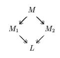
reducible). Normal order reduction is a call-by-name evaluation strategy. M —» M1 and M —» M2
M1 —» L and M2 —» L
Let us suppose to have a generic term M, and let us suppose it has two normal forms N and N'. It means that M —» N and M —» N' Let us now apply the Confluence theorem. Then there exists a term Q such that: N —» Q and N' —» Q But N and N' are in normal form, then they have not any redex. So, it necessarily means that N —» Q in 0 steps and hence that N ≡ Q.
The above result is a very important one for programming languages, since it ensures that if we implement the same algorithm in Scheme and in Haskell, the functions we obtain give us the very same result (if any), even if Scheme and Haskell are functional languages that use very different reduction strategies. In the syntax of the λ-calculus we have not considered primitive data types (the natural numbers, the booleans and so on), or primitive operations (addition, multiplication and so on), because they indeed do not represent really primitive concepts. As a matter of fact, we can represent them by using the essential notions already formalized in the λ-calculus, namely variable, application and abstraction.
Defining recursive functions In the syntax of the λ-calculus there is no primitive oparation that enables us to give names to lambda terms. However, that of giving names to expressions seems to be an essential features of programming languages in order to define functions by recursion, like in Scheme (define fact (lambda (x) (if (= x 0) 1 (* x (fact (- x 1)))))) or in Haskell fact 0 = 1 fact n = n * fact (n-1) |