The λ-calculus and computation theory

   The Lambda-calculus is the computational model the functional languages are based on.
It is a very simple mathematical formalism. In the theory of the λ-calculus one is enabled to formalize, study and investigate properties and notions common to all the functional languages, without being burdened by all the technicalities of actual languages, useless from a theoretical point of view.
In a sense, the λ-calculus it is a paradigmatic and extremely simple functional language.

The concepts the Lambda-calculus is based on are those that are fundamental in all functional programming languages:

variable         ( formalisable by   x, y ,z,…)
abstraction (anonymous function)    (formalisable by   λx.M   
                                                       where M is a term and x a variable)
application    (formalizable by  MN, where M and N are terms )

We have seen that these are indeed fundamental notions in functional programming. It seems, however, that there are other important notions: basic elements, basic operators and the possibility of giving names to expressions.
Even if it could appear very strange, this notions actually are not really fundamental ones: they can be derived from the first ones.
This means that our fucntional computational model can be based on the concepts of variable, functional abstracion and application alone.
Using the formalization of these three concepts we form the lambda-terms. These terms represent both programs and data in our computational model (whose strenght in fact strongly depends on the fact it does not distinguish between "programs" and "data".)

   The formal definition of the terms of the Lambda-calculus (lambda-terms) is given by the following grammar:

Λ ::= X | (ΛΛ) | λX.Λ

where Λ stands for the set of lambda-terms and X is a metavariable that ranges over the (numerable) set of variables (x, y, v, w, z, x2, x2,...)
Variable and application are well-known concepts, but what is abstraction?
Abstraction is needed to create anonymous functions (i.e. functions without a name). We have seen that being able to specify an anonymous function is very important in fucntional programming, but it is also important to be able to associate an identifier to an anonymous function. Nonetheless we can avoid to introduce in our model the notion of "giving a name to a function". You could ask: how is it possible to define a function like fac without being able to refer to it trought its name??? Believe me, it is possible!.

The term λx. M represents the anonymous function that, given an input x, returns the "value" of the body M.
Other notions, usually considered as primitive, like basic operators (+, *, -, ...) or natural numbers, are not strictly needed in our computational model (indeed they can actually be treated as derived concepts.)

Bracketing conventions

For readability sake, it is useful to abbreviate nested abstractions and applications as follows:

(λx₁.(λx₂. ... . (λx_n.M) ... )    is abbreviated by    (λx₁x₂ ... x_n.M)

( ... ((M₁M₂)M₃) ... M_n)    is abbreviated by    (M₁M₂M₃ ... M_n)

We also use the convention of dropping outermost parentheses and those enclosing the body of an abstraction.

Example:

(λx.(x (λy.(yx))))     can be written as     λx.x(λy.yx)

In an abstraction λx.P, the term P is said to be the scope of the abstraction.
In a term, the occurrence of a variable is said to be bound if it occurs in the scope of an abstraction (i.e. it represents the argument in the body of a function).
It is said to be free otherwise.

These two concepts can be formalized by the following definitions.

Definition of bound variable
We define BV(M), the set of the Bound Variables of M, by induction on the term as follows:

BV(x) = Φ (the emptyset)
BV(PQ) = BV(P) U BV(Q)
BV(λx.P) = {x} U BV(P)

Definition of free variable
We define FV(M), the set of the Free Variables of M, by induction on the term as follows:

FV(x) = {x}
FV(PQ) = FV(P) U FV(Q)
FV(λx.P) = FV(P) \ {x}

Substitution

The notation M [L / x] denotes the term M in which any free (i.e. not representing any argument of a function) occurrence of the variable x in M is replaced by the term L.

Definition of substitution (by induction on the structure of the term)
1. If M is a variable (M = y) then:

y [L/x] ≡	{	L    if  x=y
		y    if  x≠y

2. If M is an application (M = PQ) then:

PQ [L/x] = P[L/x] Q[L/x]

3. If M is a lambda-abstraction (M = λy.P) then:

λy.P[L/x] ≡	{	λy.P    if  x=y
		λy.(P [L /x])    if  x≠y

Notice that in a lambda abstraction a substitution is performed only if the variable to be substituted is free.

Great care is needed when performing a substitution, as the following example shows:

Example:

Both of the terms   (λx.z)    and    (λy.z)    obviously represent the constant function which returns z for any argument

Let us assume we wish to apply to both of these terms the substitution [x / z] (we replace x for the free variable z). If we do not take into account the fact that the variable x is free in the term x and bound in (λx.z) we get:

(λx.z) [x / z]  =>  λx.(z[x / z])  =>  λx.x     representing the identity function
(λy.z) [x / z]  =>  λy.(z[x/ z])  =>  λy.x     representing the function that returns always x

This is absurd, since both the initial terms are intended to denote the very same thing (a constant function returning z), but by applying the substitution we obtain two terms denoting very different things.

Hence a necessary condition in order the substitution M[L/x] be correctly performed is that free variables in L does not change status (i.e. become not free) after the substitution. More formally: FV(L) and BV(M) must be disjoint sets.
Such a problem is present in all the programming languages, also imperative ones.

Example:

Let us consider the following substitution:

(λz.x) [zw/x]

The free variable z in the term to be substituted would become bound after the substitution. This is meaningless. So, what it has to be done is to rename the bound variables in the term on which the substitution is performed, in order the condition stated above be satisfied:

(λq.x) [zw/x]

  now, by performing the substitution, we correctly get: (λq.zw)

The example above introduces and justifies the notion of alpha-convertibility

The notion of alpha-convertibility

A bound variable is used to represent where, in the body of a function, the argument of the function is used. In order to have a meaningful calculus, terms which differ just for the names of their bound variables have to be considered identical. We could introduce such a notion of identity in a very formal way, by defining the relation of α-convertibility. Here is an example of two terms in such a relation.

λz.z  =_α λx.x

We do not formally define here such a relation. For us it is sufficient to know that two terms are α-convertible whenever one can be obtained from the other by simply renaming the bound variables.
Obviously alpha convertibility mantains completely unaltered both the meaning of the term and how much this meaning is explicit. From now on, we shall implicitely  work on λ-terms modulo alpha conversion. This means that from now on two alpha convertible terms like λz.z and λx.x are for us the very same term.

Example:

(λz. ((λt. tz) z)) z

All the variables, except the rightmost z, are bound, hence we can rename them (apply α-conversion). The rightmost z, instead, is free. We cannot rename it without modifying the meaning of the whole term.

It is clear from the definition that the set of free variables of a term is invariant by α-conversion, the one of bound variables obviously not.

The formalization of the notion of computation in λ-calculus:  The Theory of β-reduction

   In a functional language to compute means to evaluate expressions, making the meaning of a given expression more and more explicit. Up to now we have formalized in the lambda-calculus the notions of programs and data (the terms in our case). Let us see now how to formalize the notion of computation. In particular, the notion of "basic computational step".
We have noticed in the introduction that in the evaluation of a term, if there is a function applied to an argument, this application is replaced by the body of the function in which the formal parameter is replaced by the actual argument.
So, if we call redex any term of the form (λx.M)N, and we call M[N/x] its contractum, to perform a basic computational step on a term P means that P contains a subterm which is a redex and that such a redex is replaced by its contractum (β-reduction is applied on the redex.)
The relation between redexes and their contracta is called notion of β-reduction, and it is represented as follows.

The notion of β-reduction

(λx.M) N →_β M [N/x]

A term P β-reduces in one-step to a term Q if  Q can be obtained out of P by replacing a subterm of P of the form (λx.M)N by M[N/x]
 

Example:

If we had the multiplication in our system, we could perform the following computations

(λx. x*x) 2  =>  2*2   =>  4

here the first step is a β-reduction; the second computation is the evaluation of the multiplication function. We shall see how this last computation can indeed be realized by means of a sequence of basic computational steps (and how also the number 2 and the function multiplication can be represented by λ-terms).

Strictly speaking, M → N means that M reduces to N by exactly one reduction step. Frequently, we are interested in whether M can be reduced to N by any number of steps.

we write    M —» N     if     M → M₁ → M₂ → ... → M_k ≡ N    (K ≥ 0)

It means that M reduces to N in zero or more reduction steps.

Example:

((λz.(zy))(λx.x)) —» y

Normalization and possibility of non termination

Definition
If a term contains no β-redex, it is said to be in normal form.
Example:

λxy.y and xyz   are in normal form.

A term is said to have a normal form if it can be reduced to a term in normal form.
Example:

(λx.x)y   is not in normal form, but it has the normal form  y

Definition:
A term M is normalizable (has a normal form, is weakly normalizable) if there exists a term Q in normal form such that

M —» Q

A term M is strongly normalizable, if there exists no infinite reduction path out of M. That is, any possible sequence of β-reductions eventually leads to a normal form. 
 

Example:

(λx.y)((λz.z)t)

is a term not in normal form, normalizable and strongly normalizable too. In fact, the only two possible reduction sequences are:

1. (λx.y)((λz.z) t) → y

2. (λx.y)((λz.z) t) → (λx.y) t) → y

To normalize a term means to apply reductions until a normal form (if any) is reached. Many λ-terms cannot be reduced to normal form. A term that has no normal form is

(λx.xx)(λx.xx)

This term is usually called Ω.

Although different reduction sequences cannot lead to different normal forms, they can produce completely differend outcomes: one could terminate while the other could "run" forever. Typically, if M has a normal form and admits an infinite reduction sequence, it contains a subterm L having no normal form, and L can be erased by some reductions. The reduction

(λy.a)Ω → a

reaches a normal form, by erasing the Ω. This corresponds to a call-by-name treatment of arguments: the argument is not reduced, but substituted 'as it is' into the body of the abstraction.
Attempting to normalize the argument generates a non terminating reduction sequence:

(λy.a)Ω →(λy.a)Ω → ...

Evaluating the argument before substituting it into the body correspons to a call-by-value treatment of function application. In this examples, a call-by-value strategy never reaches the normal form.

Some important results of β-reduction theory

   The normal order reduction strategy consists in reducing, at each step, the leftmost outermost β-redex. Leftmost means, for istance, to reduce L (if it is reducible) before N in a term LN. Outermost means, for instance, to reduce (λx.M) N before reducing M or N (if reducible). Normal order reduction is a call-by-name evaluation strategy.

Theorem (Standardization)
If a term has a normal form, it is always reached by applying the normal order reduction strategy.

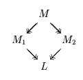
Theorem (Confluence)
If we have terms M, M₁ and M₂ such that:

M —» M₁    and    M —» M₂

then there always exists a term L such that:

M₁ —» L    and    M₂ —» L

That is, in diagram form:

 

Corollary (Uniqueness of normal form)
If a term has a normal form, it is unique.

Proof:

Let us suppose to have a generic term M, and let us suppose it has two normal forms N and N'. It means that

M —» N    and    M —» N'

Let us now apply the Confluence theorem. Then there exists a term Q such that:

N —» Q    and    N' —» Q

But N and N' are in normal form, then they have not any redex. So, it necessarily means that

N —» Q   in 0 steps

and hence that N ≡ Q.
Analogously we can show that N' ≡ Q. It is then obvious that   N ≡ N'.

The above result is a very important one for programming languages, since it ensures that if we implement the same algorithm in Scheme and in Haskell, the functions we obtain give us the very same result (if any), even if Scheme and Haskell are functional languages that use very different reduction strategies.

In the syntax of the λ-calculus we have not considered primitive data types (the natural numbers, the booleans and so on), or primitive operations (addition, multiplication and so on), because they indeed do not  represent really primitive concepts. As a matter of fact, we can represent them by using the essential notions already formalized  in the λ-calculus, namely variable, application and abstraction.

The theory of β-conversion

It is possible to formalize the notion of computational equivalence of programs into the lambda calculus. This is done by introducing the relation of β-conversion among λ-terms, denoted by M =_β N
Informally, we could say that two terms are β-convertible when they "represent the same information": actually if one can be transformed into the other by performing zero or more β-reductions and β-expansions.
(A β-expansion being the inverse of a reduction:    P[Q/x] ← (λx.P)Q  ) .
We shall not treat the theory of β-conversion in our course.

Representing data types and functions on them

In the syntax of the λ-calculus we have not considered primitive data types (the natural numbers, the booleans and so on), or primitive operations (addition, multiplication and so on), because they indeed do not  represent really primitive concepts. As a matter of fact, we can represent them by using the essential notions already formalized  in the λ-calculus, namely variable, application and abstraction (we do not provide any example here, but refer to [PS]). Even more, it is possible to represent in the lambda-calculus any computable function (notice that we do not use lambda-terms just to define mathematical functions, but to represent particular algorithms to compute mathematical functions).

Representing recursive algorithms

In the syntax of the λ-calculus there is no primitive operation that enables us to give names to lambda terms. However, that of giving  names to expressions seems to be an essential features of programming languages in order to define programs by recursion, like in Scheme

(define fact (lambda (x) (if (= x 0) 1 (* x (fact (- x 1))))))

or in Haskell

fact 0 = 1

fact n = n * fact (n-1)

Then, in order to define recursive algorithms in the λ-calculus, it would seem essential to be able to give names to expressions, so that we can recursively refer to them.
Surprisingly enough, however, that's not true at all! In fact, we can represent recursive functions in the lambda-calculus by using the few ingredients we have already at hand, exploiting the concept of fixed point.
The notion of fixed point can be represented in the lambda calculus through terms like

λf. (λx. f(xx)) (λx. f(xx))

(this term is traditionally called Y)
In fact, for any term M we have that M(YM)=_βYM
If we look at M as a function (since we can apply terms to it), the term YM is then a fixed point of M (a fixed point of a function f:D->D being an element d of D such that f(d)=d).
From fixed points we can derive the notion of recursion in the lambda calculus: in fact, intuitively, what is the function factorial? it is the function such that

factorial = λx. if (x=0) then 1 else (x*factorial(x-1))

this means that the function factorial is the fixed point of

λf. λx. if (x=0) then 1 else (x*f(x-1))

So, recursive algorithms can be represented in the lambda-calculus by means of fixed points (and hence by using terms like Y, called fixed-point combinators.) In [PS] it is discussed more precisely how to use fixed-point combinators in order to represent recursive algorithms. In particular by using a combinator different from Y, namely the combinator Θ.
After stydying fixed-point combinators in [PS] one could check that also the following term (Klop's combinator) is actually a fixed-point combinator:
££££££££££££££££££££££££££
where £ is the lambda term
λabcdefghijklmnopqstuvwxyzr.(r(thisisafixedpointcombinator))

 Reduction strategies

One of the aspects that characterizes a functional programming language is the reduction strategy it uses. Informally a reduction strategy is a "policy" which chooses a β-redex , if any, among all the possible ones present in the term. It is possible to formalize a strategy as a function, even if we do not do it here.

Let us see, now, same classes of strategies.

Call-by-value strategies
These are all the strategies that never reduce a redex  when the argument  is not a value.
Of  course we need to precisely formalize what we intend for "value".
In the following example we consider a value to be a lambda term in normal form.

Example:

Let us suppose to have:

((λx.x)((λy.y) z)) ((λx.x)((λy.y) z))

A call-by-value strategy never reduce the term (λx.x)((λy.y) z) because the argument is not a value. In a call-by-value strategy , then, we can reduce only one of the redex underlined.

Scheme uses a specific call-by-value strategy, and a particular notion of value.
Informally, up to now we have considered as "values" the terms in normal form. For Scheme, instead, also a function is considered to be a value (an expression like λx.M, in Scheme, is a value).
Then, if we have

(λx.x) (λz.(λx.x) x)

The reduction strategy of Scheme first reduces the biggest redex (the whole term), since the argument is considered to be a value (a function is a value for Scheme). After the reduction the interpreter stops, since the term λz.((λx.x) x) is a value for Scheme and hence cannot be further evaluated.


Call-by-name strategies
These are all the strategies that reduce a redex without checking whether its argument is a value or not. One of its subclasses is the set of lazy strategies. Generally, in programming languages a strategy is lazy if it is call-by-name and reduces a redex only if it's strictly necessary to get the final value (this strategy is called call-by-need too). One possible call-by-name strategy is the leftmost-outermost one: it takes, in the set of the possible redex, the leftmost and outermost one.

Example:

Let us denote by I the identity function and let us consider the term:

(I (II)) ( I (II))

the leftmost-outermost strategy first  reduces the underlined redex.

We have seen before that the leftmost-outermost strategy is very important since, by the Standardization Theorem, if a term has a normal form, we get it by following such a strategy. The problem is that the number of reduction steps is sometimes greater then the strictly necessary ones.


If a language uses a call-by-value strategy, we have to be careful because if an expression has not normal form, the search could go on endlessly.